July 2024

“A picture is worth a thousand words”
(or thousands of chemical reactions)
 

     The beta version of Kintecus 2025 has been released. This version can graphically display your chemical network in a myriad of ways by simple inclusion of a command line switch, "-chemnet". Many examples are given in the documentation. This version also combines the internal, automatic illegal loop identification with the graphical display allowing easy highlighting of illegal loops. Full description is in the documentation in the zip file located on the Beta page ( BETA page ) or click here to download it now:
 Click Here to download the Kintecus 2025 zip file

Shown below are just a few of the possible plethora of graphic network outputs one can now create:

The below panel of four cells show just a few ways to view the Enzyme Inhibition Model that comes with Kintecus. The manual at the Beta part of this website describes exactly the method to get to these plots. They all show the same exact chemical mechanism but with different filters and methods.

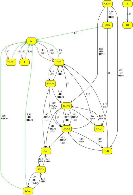
Shown below is a larger chemical model. The Kintecus-ChemNet picture is a representation of the “ Photochemical Chlorate–Iodide Clock Reaction", Romulo O. Pires and Roberto B. Faria, Inorg. Chem. 2022

Shown below is a representation of the H2-O2 Combustion mode:

The new Kintecus Chemnet feature also automatically highlights illegal loops according to Chemical Mechanism validation by David M. Stanbury and Dean Hoffman; "Systematic Application of the Principle of Detailed Balancing to Complex Homogeneous Chemical Reaction Mechanisms”; J. Phys. Chem A; 2019; 123, p5436-5445 and references therein.

Shown below are the seven simple test cases of illegal loops in the above stated paper that are automatically highlighted as illegal :

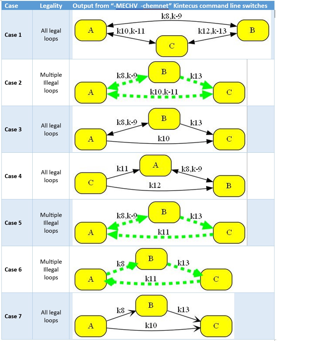
Using "-MECHV" (Mechanism Validation) with "-chemnet" shows illegal loops shown in Figure 1 in Stanbury and Hoffman 2019, J.Phys Chem. One can view the Kintecus text output for full details on this illegal loop as described in the “Mechanism Validation” Chapter in the Kintecus Manual.

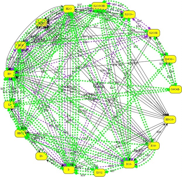
Another chemical mechanism with many types of illegal loops as highlighted:

The manual located in the Beta part (click here BETA ) has these examples, how to get to them and many, many more sample plots.

Sept 2022

Kintecus version 2021 has been released. For full details please see the What's New page:

• *NEW* For accurate chemical mechanism determination and rate constant fitting and regression, all methods listed in Stanbury and Hoffman's 2019 paper "Systematic Application of the Principle of Detailed Balancing to Complex Homogeneous Chemical Reaction Mechanisms" are NOW included in Kintecus. It appears that given a valid chemical mechanism, such a mechanism might be invalid even though the chemical mechanism may make "chemical sense". Kintecus will perform this analysis thoroughly and automatically within itself simply by adding the "-MECHV" switch on the Kintecus command line! Much more details in the manual....
   
• The option of holding concentrations/temperatures/pressure constant between datasets for global regression runs. In earlier versions of Kintecus, one could set initial conditions for each experimental dataset. These initial conditions could change during a global regression run. One can now hold this initial condition constant for each experimental dataset. For example, suppose one performed regression with many datasets with different initial conditions for each experiment (such as pH). In that case, one can now set pH values (or temperature or any other value) to different starting constant values for each run in the initial condition file, and that value will not change. It is possible to have different constant initial values for each regressed.
   
•  A new "validate" feature. This feature will allow one to compare a single Kintecus run against an external synthetic/experimental dataset. This feature (invoked by adding the "-validate:<datafile name>" flag on the command line) will force Kintecus to match exactly all timings and conditions against this externally calculated or measured dataset and produce a comparable output with statistics on that fit. This is primarily for machine learning programs to compare their output against Kintecus' output. This validate feature should be used in conjunction with the mechanism validation feature to improve ML/DL models.
   
• The NEW Jet Propulsion Laboratory multi-parameter fit the Troe expression for atmospheric, gas, combustion chemistry. Please see section 2 in the JPL Evaluation #19, 2019 (http://jpldataeval.jpl.nasa.gov/download.html). For 2019, JPL has performed a complete revision on some of these fits.
   
• The Kintecus Workbench has been expanded to include many more example models (some published), tools, examples, and other codes (such as Atropos). See "What's New" for a picture of the Kintecus Workbench Menu system!
   
• Water Purification and Analysis files are constantly being added to the package. Please check the latest package distribution for the contents.
  (Package 3 is available for download as of Sept 2022)
   
• More features! See What's New for more details!

Sept 2022

Kintecus V2021, Version 3 Package Distribution
=========================================

- Water Purification and Analysis files are constantly being added to the package. Please check the latest package distribution for the contents.
(Package 3 is available for download as of Sept 2022)
- Epidemiology models have been added under "Other" on Workbench menu.
- More minor updates to the Kintecus Manual.



July 24th 2022

Kintecus V2021, Version 2 Package Distribution
=========================================

[*] (a) if the last defined species in your species worksheet was used in a User Defined Function, Kintecus will not be able to find it. This is fixed
(b) One should now be able to use cations/anions in User Defined Functions without errors.
In general, one should try and use an internal Kintecus kinetic equation rather defining your own as the internal ones are 100x (10,000%) faster.

October 7th 2021

“Kintecus 2021” has been released:
=======================================================

Manual for Kintecus V2021. New additions are highlighted in yellow.

 *NEW* For accurate chemical mechanism determination, rate constant fitting, and regression, the application of all methods listed in Stanbury and Hoffman's 2019 paper "Systematic Application of the Principle of Detailed Balancing to Complex Homogeneous Chemical Reaction Mechanisms" is now fully included in Kintecus. It appears that given a valid chemical mechanism, such a mechanism might be invalid even though the chemical mechanism may make "chemical sense." Kintecus can perform this analysis thoroughly and automatically within itself simply by adding the "-MECHV" switch on the Kintecus command line! This new feature will help design more accurate, and long-term ML/DL chemical models for CFD runs. BUT WAIT! There's MORE! The Installation of "R" and the Mathematica systems are NOT REQUIRED!
In some cases, Kintecus can out-predict the Mathematica system in linear programming/optimization methods[*].

What else is also NEW in Kintecus 2021:
=======================================================
1) The option of holding concentrations/temperatures/pressure constant between datasets for global regression runs. In earlier versions of Kintecus one could set initial conditions for each experimental dataset. These initial conditions could change during a global regression run. One can now hold this initial condition constant for each experimental dataset. For example, if one was performing regression with many datasets with different initial conditions for each experiment (such as pH), one can now set pH values (or temperature or any other value) to different starting constant values for each run in the initial condition file and that value will not change. It is possible to have different constant initial values for each regressed experimental dataset.
2) The NEW Jet Propulsion Laboratory multi-parameter fit to the Troe expression for atmospheric, gas, combustion chemistry. Please see section 2 in the JPL Evaluation #19, 2019 (http://jpldataeval.jpl.nasa.gov/download.html). For 2019, JPL has performed a complete revision on some of these fits.
3) The amount of chemical families and families of species has been substantially upgraded. One can have many more families of species (such as ROH=[C2H5OH]+[C3H7OH]+[C4H9OH]+... ) and have many more terms for each one.
4) A new “validate” feature. This feature will allow one to compare a single Kintecus run against an external synthetic/experimental dataset. This feature (invoked by adding
 the “-validate:<datafile name>” flag on the command line) will force Kintecus to match exactly all timings and conditions against this externally calculated or measured dataset and produce a comparable output with statistics on that fit. This is primarily for machine learning programs to compare their output against Kintecus’ output. This should be used in conjunction with the mechanism validation feature to improve ML/DL models.
 

[*] Private communication and testing with Dr. Stanbury in 2020.
--------------------------------------------------------------------------------------
MORE RELEASE NOTES (that nobody reads):

**********************************************************
1. VIRUS RANSOMWARE! Note that Kintecus will write to
C:\Kintecus\ folder. You might need to tell your
anti-virus software to turn off ransomware protection
on "C:\Kintecus" and/or place the "kintecus.exe" file
as "safe" or turn off Advanced Threat Defense options.
THERE ARE MORE OPTIONS, PLEASE SEE BELOW! ----vvv

2. The old Excel "xls" files have been moved to
the "OLD_EXCEL_XLS_KINTECUS_FILES" folder.
Most Kintecus-Excel worksheets have been updated to
xlsm files. If you need an older Kintecus-Excel worksheet, they
are in "OLD_EXCEL_XLS_KINTECUS_FILE" folder.

3. - KINTECUS INSTALL PATH RESET TO "C:\KINTECUS\"
The default installation path for Kintecus is now at
"C:\Kintecus\"
This was decided to alleviate the write permission
problems Windows7/10 users were experiencing.
The previous default path of
C:\Program Files\Kintecus would
cause write access errors to that directory.
**********************************************************

VIRUS SOFTWARE PREVENTING KINTECUS TO RUN?
==================================================
The Kintecus package is scanned by several anit-virus software programs before distribution.
You can always run a full gauntlet of 60+ virus scans by using Google's free VirusTotal website too!

Here are some options to get Kintecus or Kintecus to run under some pesky anti-virus code:
-------------------------------------------------------------------------------------------
(1) It is possible that your anti-virus software is preventing the Kintecus executable or Kintecus_Workbench executable or the “cmd.exe” Windows program from running. Most anti-virus software have a “safe” list or an exception list. Please add those executables to that list. This can also happen from anti-Ransomware software that is preventing Kintecus from writing to the “..\Kintecus\” folder. Please remove such protections on that folder and executable or enable the above executables to a safe list.

(2) Even if you have zero anti-virus software installed, Microsoft has an internal anti-virus procedures in Excel that can prevent some Kintecus-Excel macros from running.
You can set all Kintecus-Excel Workbooks to Trusted by setting the directory "C:\Kintecus" as a "Trust Location" in the Excel Trust Center. You can do this by going to File==>Options==>"Trust Center", click the "Trust Center Settings..." button, click "Trust Locations", click "Add new location...", click "Browse", select the "C:\Kintecus\" directory (or whatever PATH you installed Kintecus), click 'OK', then click OK again. You should now fully run all Kintecus-Excel Workbooks with no interference from Excel errors.
You can also see "https://support.microsoft.com/en-us/office/add-remove-or-change-a-trusted-location-7ee1cdc2-483e-4cbb-bcb3-4e7c67147fb4" for more details.

(3) If you are still having trouble running Kintecus in Excel, then don't run Kintecus in Excel!
Please see the section "Run Kintecus Outside of Excel and/or Run Many Copies of Kintecus on one PC ?"
inside the manual or look below:

-------------------------------------------------------------------------------------------------
How to Run Kintecus Outside of Excel and/or Run Many Copies of Kintecus on one PC ?
-------------------------------------------------------------------------------------------------
This part explains how to run Kintecus using the MODEL/SPECIES/PARM/FITDATA/etc worksheets in Excel without having Excel constantly open up, waste cpu cycles and constantly annoy you as your Kintecus simulation runs.
Click the Windows Start Button in the button, left hand corner of the screen and type “cmd” or "command" and press enter. A console window should pop up on the screen. Alternatively, hold the Windows key (usually the key is at the bottom left of the keyboard, in between the CTRL and ALT keys) and tap the "x" key. A menu will pop up, select or "Command" or "run" (and type “cmd” or “command”), a new console should pop up.

A) Once you are in the console window (or PowerShell window), type "cd C:\Kintecus" or where ever you have Kintecus installed.
B) In the Excel Window, click on "CONTROL" tab, click "RUN", once Kintecus starts, stop it with "ctrl-c" (hold ctrl key and tap the "c" key) or ctrl-break (hold ctrl key and tap the Pause/Break key). The reason for this step is that once you press the RUN button, the Kintecus-Excel VBA macros will output all your worksheets as input files for Kintecus.
C) In the same "CONTROL" worksheet, click on the contents of the "Kintecus Switches" cell (A12) and select COPY (right click, select Copy)
D) Click in the console/command line window, in PowerShell/command type "./kintecus". In command console, just type "kintecus" (don’t press enter yet!)
E) Hold down the CTRL key and type "V" (for paste) and press ENTER. This should paste your Kintecus switches from cell A12 on the CONTROL worksheet into the command line.
F) Kintecus is now running outside of Excel using all your inputs from the Excel Worksheet. Once Kintecus is finished, click the “Plot Results” button located on the CONTROL worksheet. Also, note that you can copy the entire Kintecus folder into a new directory (C:\Kintecus2\), change the “Kintecus Path” located on the CONTROL worksheet, then change one or two parameters in the Kintecus-Excel worksheet and perform the same steps above. You will be running two different Kintecus simulations/optimizations at the same time. Repeat as much as necessary assuming you have enough cores on your cpu.
 

December 13th 2020

Kintecus V2021 Beta2 released. Updated executable, Kintecus-Excel workbooks and Kintecus manual at

www.kintecus.com/newpage15.htm

The new additions have been highlighted in yellow in the new Kintecus V2021 Manual.

February 17th, 2019

Kintecus V6.80 released:

• The ultra-accurate standard error calculation of fits known as bootstrapping now supports Global/local regression datasets for both global and local variable regressions with/without equation constraints with/without multiple datasets with/without uneven time steps/unlimited data points with/without global/local initial conditions and with/without parameter constraints. This version comes with several published models in ACS/Elsevier journals. Kintecus is the only code in the world that can do this.
  You longer need Matlab, nor Origin, nor Igor, nor JMP to workup your data and/or painstakingly create special scripts to analyze your data.
  Please see the "Global Regression Analysis/Many Datasets+Init Conditions+Accurate Error Analysis 1" in the Kintecus Workbench program (or click on the Kintecus-Excel worksheet "Fe(VI)+ABTS_Fe(IV)_involved_multiple_fitting_20180729_10mM borate_pH=7_ks3=1e6.xlsm"). This method was recently extensively utilized in the ACS journal:
  "Huang, Z.-S.; Wang, L.; Liu, Y.-L.; Jiang, J.; Xue, M.; Xu, C.-B.; Zhen, Y.-F.; Wang, Y.-C.; Ma, J., Impact of Phosphate on Ferrate Oxidation of Organic Compounds: An Underestimated Oxidant. Environ. Sci. Technol. 2018, 52, (23), 13897-13907."

• A few enahancments:A fix for thermodynamic databases that have coefficients with positive exponents represented by a space such as "1.234E 32" (it should be read in as 1.234E+32) or "9.874E 12" (9.874E+12) The older versions of Kintecus would read them as "1.234" and "9.874". Note that exponents with lower case "e" such as   "1.234e 32" were always read in correctly by Kintecus.

• bug corrections for user defined constraints in regressions, other bug fixes.

• The Kintecus Workbench has been expanded to include many more example models (some published), tools, examples and other codes (such as Atropos):